Visualise and debug the functions

In this tutorial, we are going to visualise Rational Functions.

Visualise

First let’s create some rational functions

from rational.torch import Rational

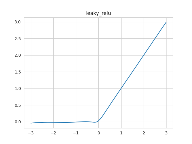
rat_l = Rational("leaky_relu")
rat_s = Rational("sigmoid")
rat_i = Rational("identity")

Then let’s call the show() method to visualize it.

rat_l.show()

We can also visualise every instanciated rational function. They are stored in the list attribute of the Rational module:

print(Rational.list)
# [Rational Activation Function A) of degrees (5, 4) running on cuda 0x7f778678b700
# , Rational Activation Function A) of degrees (5, 4) running on cuda 0x7f778678b1c0
# , Rational Activation Function A) of degrees (5, 4) running on cuda 0x7f77851fb5b0
# ]

They correspond to the 3 rational functions we have instanciated. To see them all, use the class method show_all():

Rational.show_all()

The visualisation of the functions is based on Snapshot. When we call show() or show_all(), a Snapshot is created and displayed.

You can capture snapshot at a specific point during your experiment and it will be stored in snapshot_list of the specific rational function:

print(rat_l.snapshot_list)
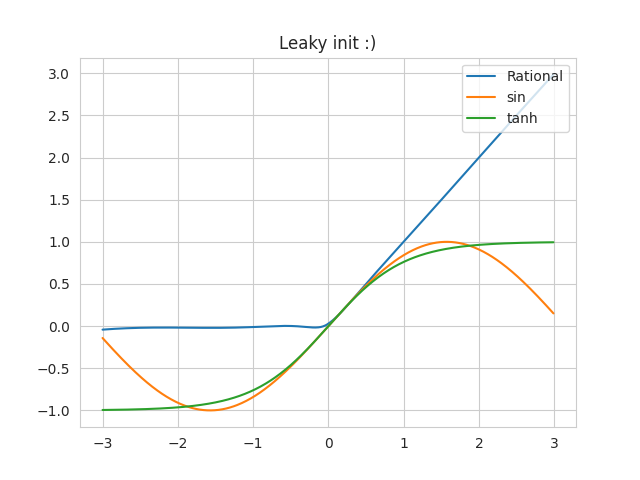
rat_l.capture(name="Leaky init :)")
print(rat_l.snapshot_list)
# []
# [Snapshot (Leaky init :))]

Now you can use the show() method to display the captured snapshot. You can even compare it to other functions by using other_func.

import torch
rat_l.snapshot_list[0].show(other_func=[torch.sin, torch.tanh])

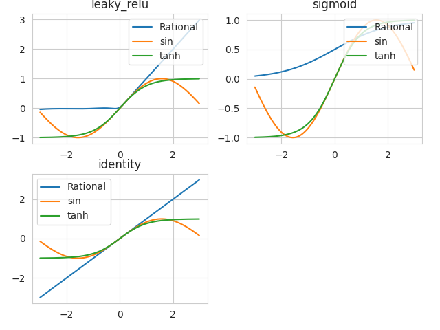
You can, of course pass this parameter to the show_all() function

Rational.show_all(other_func=[torch.sin, torch.tanh])

we can also directly save the graphs instead of displaying it, by using the export_graph() and classmethod export_graphs() of our rational.

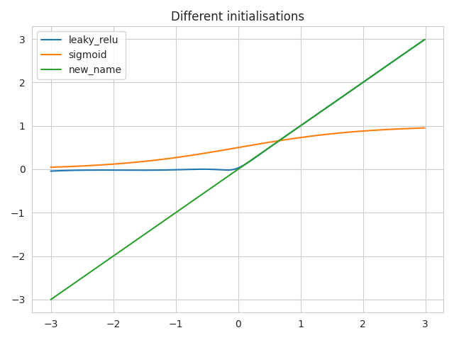
You can also give your own axis to visualise all instanciated function on the same axis or chery pick the functions you want to vizualize on the same graph:

import matplotlib.pyplot as plt
import seaborn as sns

with sns.axes_style("whitegrid"):
    ax = plt.gca()

rat_i.func_name = "new_name"

for rat in Rational.list:
    rat.show(title="Different initialisations", axis=ax)
plt.legend()
plt.show()

Rational.show_all(title="Different initialisations", axes=ax)  # equivalent

Visualise the functions’ evolutions through learning

We can also look at the evolution of the functions, while learning. To do so, we capture snapshots at different epochs. Let’s define have 3 rational functions, initialized differently, and have them learn the sinus function. We capture at different epochs.

from rational.torch import Rational
import torch

rat_l = Rational("leaky_relu")
rat_s = Rational("sigmoid")
rat_i = Rational("identity")

device = "cuda" if torch.cuda.is_available() else "cpu"
criterion = torch.nn.MSELoss()

optimizers = [torch.optim.Adam(rat.parameters(), lr=0.01)
              for rat in Rational.list]

capturing_epochs = [0, 1, 2, 4, 8, 16, 32, 64, 99, 149, 199]
for epoch in range(200):
    for (rat, optimizer) in zip(Rational.list, optimizers):
        inp = ((torch.rand(10000)-0.5)*5).to(device)
        exp = torch.sin(inp)
        optimizer.zero_grad()
        out = rat(inp)
        loss = criterion(out, exp)
        loss.backward()
        optimizer.step()
    if epoch in capturing_epochs:
        Rational.capture_all(f"Epoch {epoch}")

Rational.export_evolution_graphs(other_func=torch.sin)

We obtain a file rationals_evolution.gif:

For learnable activation functions, learning the input distribution might help a lot understand what happens within the activation functions.

For the pytorch version of Rational activations, we can use the classmethod save_all_inputs() to save the input distribution.

capturing_epochs = [0, 1, 2, 4, 8, 16, 32, 64, 99, 149, 199]
for epoch in range(200):
    for (rat, optimizer) in zip(Rational.list, optimizers):
        inp = torch.cat([torch.randn(1000)+i for i in range(-3, 4, 3)]).to(device)
        exp = torch.sin(inp)
        optimizer.zero_grad()
        if epoch in capturing_epochs:
            Rational.save_all_inputs(True)
        out = rat(inp)
        loss = criterion(out, exp)
        loss.backward()
        optimizer.step()
    if epoch in capturing_epochs:
        Rational.capture_all(f"Epoch {epoch}")
        Rational.save_all_inputs(False)

Rational.export_evolution_graphs(other_func=torch.sin)

If you want to see histograms instead of the KDE of it, you can use the use_kde of the Rational class:

Rational.use_kde = False

Use a tensorboardX SummaryWriter to plot the evolutions

You can also follow the learning of your functions by looking at evolutions of the function in a tensorboardX.SummaryWriter, to do so, give the writer to the show() or show_all() method and the evolution of the rational functions’ shapes will be provided to the tensorboard webpage.

An example code is:

from rational.torch import Rational
import torch

rat_l = Rational("leaky_relu")
rat_s = Rational("sigmoid")
rat_i = Rational("identity")

device = "cuda" if torch.cuda.is_available() else "cpu"
criterion = torch.nn.MSELoss()

optimizers = [torch.optim.Adam(rat.parameters(), lr=0.01)
              for rat in Rational.list]

capturing_epochs = [0, 1, 2, 4, 8, 16, 32, 64, 99, 149, 199]
for epoch in range(200):
    for (rat, optimizer) in zip(Rational.list, optimizers):
        inp = ((torch.rand(10000)-0.5)*5).to(device)
        exp = torch.sin(inp)
        optimizer.zero_grad()
        out = rat(inp)
        loss = criterion(out, exp)
        loss.backward()
        optimizer.step()

Provides on tensorboard webpage:

The code is taken from the `Rational_RL repository<https://github.com/ml-research/rational_rl>`_